Lab 10: Numerical Differentiation & Integration#
Examples (by instructor)#
In this lab you will practice the numerical tools from Chapter 15:
Task |
Tool |
Key syntax |
|---|---|---|
Derivative of discrete data |
|
|
Integral of discrete data |
|
|
Integral of a Python function |
|
|
Example 1: Reaction Rate from Concentration Data (np.gradient)#
In a batch reactor experiment, species A is consumed over time. We measure \(C_A\) at discrete time points and compute the reaction rate of disappearance:
np.gradient uses central differences at interior points and one-sided differences at the endpoints — automatically handling non-uniform spacing.
import numpy as np
import matplotlib.pyplot as plt
from scipy.integrate import quad, trapezoid, cumulative_trapezoid

t   = np.array([0,    10,   20,   30,   40,   50,   60  ])  # s
C_A = np.array([1.00, 0.78, 0.61, 0.48, 0.37, 0.29, 0.23])  # mol/L

# Reaction rate: r_A = -dC_A/dt
print(f"{'t (s)':>6}  {'C_A (mol/L)':>12}  {'r_A (mol/L·s)':>14}")
print("-" * 38)
for i in range(len(t)):
    print(f"  {t[i]:>4.0f}  {C_A[i]:>12.2f}  {r_A[i]:>14.4f}")

fig, axes = plt.subplots(1, 2, figsize=(11, 4))
axes[0].plot(t, C_A, 'o-', color='steelblue')
axes[0].set_xlabel('Time (s)'); axes[0].set_ylabel('$C_A$ (mol/L)')
axes[0].set_title('Concentration vs. Time')

axes[1].plot(t, r_A, 's-', color='tomato')
axes[1].set_xlabel('Time (s)'); axes[1].set_ylabel('$r_A$ (mol/L·s)')
axes[1].set_title('Reaction Rate vs. Time')
plt.tight_layout(); plt.show()
 t (s)   C_A (mol/L)   r_A (mol/L·s)
--------------------------------------
---------------------------------------------------------------------------
NameError                                 Traceback (most recent call last)
Cell In[2], line 4
      2 print("-" * 38)
      3 for i in range(len(t)):
----> 4     print(f"  {t[i]:>4.0f}  {C_A[i]:>12.2f}  {r_A[i]:>14.4f}")
      6 fig, axes = plt.subplots(1, 2, figsize=(11, 4))
      7 axes[0].plot(t, C_A, 'o-', color='steelblue')

NameError: name 'r_A' is not defined
Example 2: Heat Required from Tabulated \(C_p\) Data (trapezoid)#
A steam process requires heating from 400 K to 1000 K. Given tabulated heat capacity values, compute the enthalpy change:
trapezoid(y, x) connects adjacent data points with straight lines and sums the trapezoidal areas. Always pass x as the second argument — omitting it assumes unit spacing and gives the wrong answer when your x-axis has physical units.
# Tabulated Cp data for steam (J/mol·K)
T_data  = np.array([400,  500,  600,  700,  800,  900,  1000])  # K
Cp_data = np.array([34.3, 35.2, 36.3, 37.5, 38.6, 39.7,  40.8])  # J/mol·K

delta_H = trapezoid(Cp_data, T_data)   # J/mol
print(f"ΔH = ∫Cp dT = {delta_H:.1f} J/mol = {delta_H/1000:.3f} kJ/mol")

fig, ax = plt.subplots(figsize=(7, 4))
T_fine = np.linspace(400, 1000, 300)
ax.fill_between(T_data, Cp_data, alpha=0.25, color='steelblue', label='Trapezoid area')
ax.plot(T_data, Cp_data, 'o-', color='steelblue', linewidth=2)
ax.set_xlabel('Temperature (K)'); ax.set_ylabel('$C_p$ (J/mol·K)')
ax.set_title(f'ΔH = {delta_H/1000:.2f} kJ/mol')
ax.legend(); plt.tight_layout(); plt.show()
Warm-Up: Syntax Practice#
Short exercises to get comfortable with the four tools before the main problems.
Exercise 1 — np.gradient: velocity from position data.
Given position data sampled every 0.5 s:
\(t\) (s) |
0.0 |
0.5 |
1.0 |
1.5 |
2.0 |
2.5 |
3.0 |
|---|---|---|---|---|---|---|---|
\(x\) (m) |
0.0 |
1.4 |
2.5 |
3.3 |
3.8 |
4.0 |
4.0 |
Compute the velocity \(v = dx/dt\) at every point using np.gradient. Print the result and identify which formula (forward / central / backward) was used at each endpoint.
import numpy as np
from scipy.integrate import quad, trapezoid, cumulative_trapezoid

t = np.array([0.0, 0.5, 1.0, 1.5, 2.0, 2.5, 3.0])
x = np.array([0.0, 1.4, 2.5, 3.3, 3.8, 4.0, 4.0])

v = np.gradient(___, ___)

print("t (s):", t)
print("v (m/s):", np.round(v, 4))
Exercise 2 — trapezoid: integrate tabulated flow rate data.
A pump delivers flow at the following measured rates:
\(t\) (min) |
0 |
2 |
5 |
8 |
10 |
13 |
15 |
|---|---|---|---|---|---|---|---|
\(Q\) (L/min) |
0 |
3.1 |
5.8 |
6.4 |
6.0 |
4.2 |
2.0 |
The total volume delivered is \(V = \int_0^{15} Q(t)\,dt\).
Use trapezoid to compute the total volume in liters. Note that the time points are not equally spaced.
t_pump = np.array([0,   2,   5,   8,   10,  13,  15 ])   # min
Q      = np.array([0, 3.1, 5.8, 6.4, 6.0, 4.2, 2.0])   # L/min

V_total = trapezoid(___, ___)

print(f"Total volume delivered: {V_total:.2f} L")
Exercise 3 — quad: integrate a Python function.
The NIST Shomate equation gives the heat capacity of N₂ (298–6000 K range) as:
with \(A=26.092\), \(B=8.219\), \(C=-1.976\), \(D=0.159\), \(E=0.044\).
Use quad to compute \(\Delta H = \int_{300}^{1200} C_p(T)\,dT\) in kJ/mol. Print both the result and the error estimate returned by quad.
A, B, C, D, E = 26.092, 8.219, -1.976, 0.159, 0.044

def Cp_N2(T):
    t = T / 1000.0
    return ___   # J/mol·K

dH, err = quad(___, ___, ___)

print(f"ΔH = {dH/1000:.3f} kJ/mol")
print(f"Error estimate: {err:.2e} J/mol")
Practice Problems (by students)#
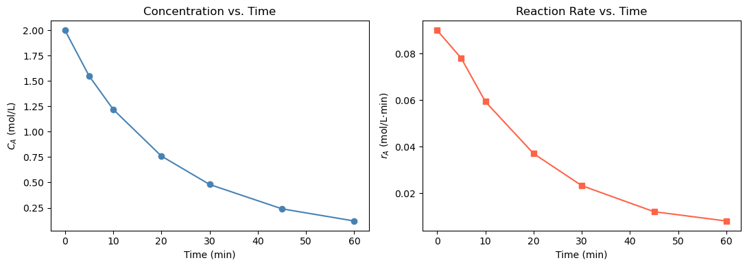
Problem 1: Batch Reactor — Rate from Concentration Data#
In a batch reactor experiment, species A undergoes a reaction of unknown order. Concentration is measured at the following times:
\(t\) (min) |
0 |
5 |
10 |
20 |
30 |
45 |
60 |
|---|---|---|---|---|---|---|---|
\(C_A\) (mol/L) |
2.00 |
1.55 |
1.22 |
0.76 |
0.48 |
0.24 |
0.12 |
The reaction rate is \(r_A = -dC_A/dt\).
(a) Use np.gradient to compute \(r_A\) at each time point. Print a table of \(t\), \(C_A\), and \(r_A\). Plot \(C_A\) vs. \(t\) and \(r_A\) vs. \(t\) side by side.
import numpy as np
import matplotlib.pyplot as plt
from scipy.integrate import quad, trapezoid, cumulative_trapezoid

t_rxn = np.array([0,    5,    10,   20,   30,   45,   60  ])  # min
C_A   = np.array([2.00, 1.55, 1.22, 0.76, 0.48, 0.24, 0.12])  # mol/L

# (a) Compute reaction rate
r_A = TODO

print(f"{'t (min)':>8}  {'C_A (mol/L)':>12}  {'r_A (mol/L·min)':>16}")
print("-" * 42)
for i in range(len(t_rxn)):
    print(f"  {t_rxn[i]:>6.0f}  {C_A[i]:>12.2f}  {r_A[i]:>16.4f}")

fig, axes = plt.subplots(1, 2, figsize=(11, 4))

axes[0].plot(t_rxn, C_A, 'o-', color='steelblue')
axes[0].set_xlabel('Time (min)')
axes[0].set_ylabel('$C_A$ (mol/L)')
axes[0].set_title('Concentration vs. Time')

axes[1].plot(t_rxn, r_A, 's-', color='tomato')
axes[1].set_xlabel('Time (min)')
axes[1].set_ylabel('$r_A$ (mol/L·min)')
axes[1].set_title('Reaction Rate vs. Time')

plt.tight_layout()
plt.show()
 t (min)   C_A (mol/L)   r_A (mol/L·min)
------------------------------------------
       0          2.00            0.0900
       5          1.55            0.0780
      10          1.22            0.0593
      20          0.76            0.0370
      30          0.48            0.0232
      45          0.24            0.0120
      60          0.12            0.0080
(b) Recompute \(r_A\) using only NumPy array operations — no np.gradient. Use:
a forward difference at the first point: \(\displaystyle\left.\frac{dC_A}{dt}\right|_0 \approx \frac{C_{A,1} - C_{A,0}}{t_1 - t_0}\)
central differences at interior points: \(\displaystyle\left.\frac{dC_A}{dt}\right|_i \approx \frac{C_{A,i+1} - C_{A,i-1}}{t_{i+1} - t_{i-1}}\)
a backward difference at the last point: \(\displaystyle\left.\frac{dC_A}{dt}\right|_{-1} \approx \frac{C_{A,-1} - C_{A,-2}}{t_{-1} - t_{-2}}\)
Print a table of \(t\), \(C_A\), and \(r_A\). Note: the endpoint values will differ slightly from part (a) because np.gradient uses a higher-order one-sided formula at the boundaries.
# (b) Compute r_A using numpy array operations (no np.gradient)
dCdt = np.zeros(len(t_rxn))

# Forward difference at the first point
dCdt[0] = TODO

# Central differences at interior points
dCdt[1:-1] = (C_A[2:] - C_A[:-2]) / (t_rxn[2:] - t_rxn[:-2])

# Backward difference at the last point
dCdt[-1] = TODO

r_A_manual = -dCdt

print(f"{'t (min)':>8}  {'C_A (mol/L)':>12}  {'r_A (mol/L·min)':>16}")
print("-" * 42)
for i in range(len(t_rxn)):
    print(f"  {t_rxn[i]:>6.0f}  {C_A[i]:>12.2f}  {r_A_manual[i]:>16.4f}")
 t (min)   C_A (mol/L)   r_A (mol/L·min)
------------------------------------------
       0          2.00            0.0900
       5          1.55            0.0780
      10          1.22            0.0527
      20          0.76            0.0370
      30          0.48            0.0208
      45          0.24            0.0120
      60          0.12            0.0080
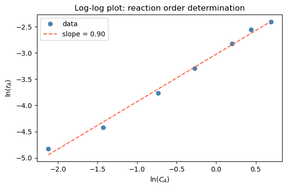
(c) To determine the reaction order, plot \(\ln(r_A)\) vs. \(\ln(C_A)\) and determine the correlation between them. Estimate the reaction order \(n\) by calculating the slope.
# (c) Log-log plot to determine reaction order
coeffs = TODO # use np.polyfit to fit ln(r_A) vs. ln(C_A)
n = TODO
print(f"Estimated reaction order: n = {n:.2f}")

fig, ax = plt.subplots(figsize=(6, 4))
ax.plot(np.log(C_A), np.log(r_A), 'o', color='steelblue', label='data')
ln_C_fit = np.linspace(np.log(C_A.min()), np.log(C_A.max()), 100)
ax.plot(ln_C_fit, np.polyval(coeffs, ln_C_fit), '--', color='tomato', label=f'slope = {n:.2f}')
ax.set_xlabel('ln($C_A$)')
ax.set_ylabel('ln($r_A$)')
ax.set_title('Log-log plot: reaction order determination')
ax.legend()
plt.tight_layout()
plt.show()
Estimated reaction order: n = 0.90
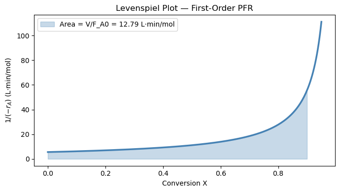
Problem 2: PFR Design — Levenspiel Integration#
A plug flow reactor processes species A via a first-order liquid-phase reaction:
The design equation is:
The analytical solution for a first-order PFR is \(V = \dfrac{F_{A0}}{k C_{A0}} \ln\!\left(\dfrac{1}{1-X_f}\right)\).
(a) Define levenspiel(X) = \(1/(-r_A(X))\) and use quad to compute \(V\) for \(X_f = 0.90\). Compare to the analytical answer and print the relative error.
import numpy as np
import matplotlib.pyplot as plt
from scipy.integrate import quad, trapezoid, cumulative_trapezoid

k    = 0.12    # 1/min
C_A0 = 1.5     # mol/L
F_A0 = 3.0     # mol/min
X_f  = 0.90

def rate_1st(X):
    return TODO

def levenspiel_1st(X):
    return 1.0 / rate_1st(X)

# (a) quad integration
integral, err = TODO
V_quad = TODO

# Analytical answer
V_exact = TODO

print(f"V (quad):       {V_quad:.4f} L")
print(f"V (analytical): {V_exact:.4f} L")
print(f"Relative error: {TODO:.2e}")

X_plot = np.linspace(0, 0.95, 300)

fig, ax = plt.subplots(figsize=(7, 4))
ax.plot(X_plot, levenspiel_1st(X_plot), 'steelblue', linewidth=2.5)

X_shade = np.linspace(0, X_f, 300)
ax.fill_between(X_shade, levenspiel_1st(X_shade), alpha=0.3, color='steelblue',
                label=f'Area = V/F_A0 = {V_quad/F_A0:.2f} L·min/mol')

ax.set_xlabel('Conversion X')
ax.set_ylabel('$1 / (-r_A)$ (L·min/mol)')
ax.set_title('Levenspiel Plot — First-Order PFR')
ax.legend()
plt.tight_layout()
plt.show()
V (quad):       38.3764 L
V (analytical): 38.3764 L
Relative error: 2.78e-15