Chapter 14: Monte Carlo Simulation

14.1 What Is Monte Carlo Simulation?

Suppose you have a bucket divided into two sections by an irregular divider — the kind of curved, uneven shape that would be painful to measure precisely.

A bucket split into Section A and Section B by an irregular divider. The question is simple: what is the area ratio A : B?

You could try to measure every curve with a ruler — tedious and error-prone. Or you could use a smarter approach: throw balls into the bucket randomly, thousands of times, then just count how many land in each section.

After throwing 80 balls uniformly at random, 40 land in each section — so the estimated area ratio is 1 : 1. With more balls, the estimate converges to the true ratio.

Because the throws are uniformly random, each ball is equally likely to land anywhere in the bucket. So the fraction that lands in Section A is proportional to its area:

\[ \frac{\text{Area A}}{\text{Total Area}} \approx \frac{N_A}{N_\text{total}} \qquad \text{as } N \to \infty \]

This is the core idea of Monte Carlo simulation — instead of computing something analytically, you sample randomly and count outcomes. The more samples you take, the more accurate the estimate.

The three-step recipe

1. Define your uncertain inputs as probability distributions

2. Draw thousands of random samples from those distributions

3. Run your model for every sample, then look at the output distribution

Why is this useful for chemical engineers?

• Uncertainty propagation: How does uncertainty in activation energy \(E_a\) affect predicted conversion?

• Process reliability: What fraction of batches will meet the purity spec given normal operating variability?

• Risk assessment: What is the probability that reactor temperature exceeds a safety limit?

• Equipment sizing: Given uncertain feed compositions, what reactor volume ensures 99% of scenarios achieve the desired conversion?

14.2 Building Intuition: Estimating π by Throwing Darts

Before tackling engineering problems, let’s build intuition with a playful classic example.

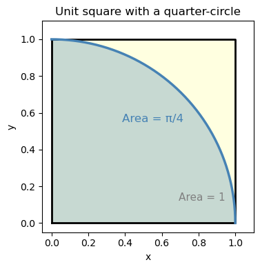
The setup: Imagine throwing darts randomly at a square dartboard. Inside the square, there’s a quarter-circle drawn in the corner. If your throws are truly random (uniform), what fraction of darts land inside the quarter-circle?

Run the cell below to see it — then we’ll work out the math.

import numpy as np
import matplotlib.pyplot as plt

fig, ax = plt.subplots(figsize=(4, 4))

# Square
ax.fill([0, 1, 1, 0], [0, 0, 1, 1], color='lightyellow', zorder=0)
ax.plot([0, 1, 1, 0, 0], [0, 0, 1, 1, 0], 'k-', linewidth=2)

# Quarter-circle region
theta = np.linspace(0, np.pi/2, 300)
ax.fill_between(np.cos(theta), np.sin(theta), 0,
                color='steelblue', alpha=0.3, label='Quarter-circle  (area = π/4)')
ax.plot(np.cos(theta), np.sin(theta), 'steelblue', linewidth=2.5)

# Labels
ax.text(0.55, 0.55, 'Area = π/4', color='steelblue', fontsize=12, ha='center')
ax.text(0.82, 0.12, 'Area = 1', color='gray',      fontsize=11, ha='center')

ax.set_aspect('equal')
ax.set_xlim(-0.05, 1.1); ax.set_ylim(-0.05, 1.1)
ax.set_xlabel('x'); ax.set_ylabel('y')
ax.set_title('Unit square with a quarter-circle')
plt.tight_layout()
plt.show()

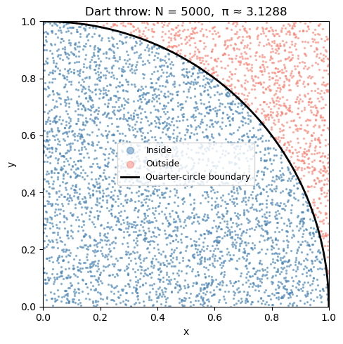
Notice that the blue darts (inside the quarter-circle) fill roughly 78% of the square — and \(\pi/4 \approx 0.785\). That’s no coincidence!

The square has area \(1 \times 1 = 1\).
The quarter-circle of radius 1 has area \(\dfrac{\pi}{4}\).

So the fraction of darts inside is: $\( \frac{\text{darts inside}}{\text{total darts}} \approx \frac{\pi/4}{1} = \frac{\pi}{4} \quad \Longrightarrow \quad \hat{\pi} \approx 4 \times \frac{\text{darts inside}}{\text{total darts}} \)$

We can use this to estimate \(\pi\) just by counting random points. Let’s do it properly with more darts.

import numpy as np
import matplotlib.pyplot as plt

# --- Step 1: Set up the random number generator ---
# Using a fixed seed so results are reproducible (same "random" numbers every run)
rng = np.random.default_rng(seed=0)

# --- Step 2: Throw random darts ---
N = 5000   # number of darts (try changing this!)

x = rng.random(N)   # x-coordinates uniformly between 0 and 1
y = rng.random(N)   # y-coordinates uniformly between 0 and 1

# --- Step 3: Check which darts land inside the quarter-circle ---
# A point (x, y) is inside the quarter-circle if x² + y² ≤ 1
inside = (x**2 + y**2) <= 1.0

# --- Step 4: Estimate π ---
pi_estimate = 4.0 * np.sum(inside) / N

print(f"Number of darts: {N}")
print(f"Darts inside quarter-circle: {np.sum(inside)}")
print(f"Fraction inside: {np.mean(inside):.4f}")
print(f"Estimated π = 4 × {np.mean(inside):.4f} = {pi_estimate:.4f}")
print(f"True π      = {np.pi:.4f}")
print(f"Error       = {abs(pi_estimate - np.pi):.4f}")

Number of darts: 5000
Darts inside quarter-circle: 3911
Fraction inside: 0.7822
Estimated π = 4 × 0.7822 = 3.1288
True π      = 3.1416
Error       = 0.0128

Visualizing the dart throw

Let’s plot the darts — blue for inside the quarter-circle, red for outside. You can see how the ratio of blue to total gives us π/4.

fig, ax = plt.subplots(figsize=(5, 5))

ax.scatter(x[inside],  y[inside],  s=2, color='steelblue', alpha=0.5, label='Inside')
ax.scatter(x[~inside], y[~inside], s=2, color='salmon',    alpha=0.5, label='Outside')

# Draw the quarter-circle boundary
theta = np.linspace(0, np.pi/2, 300)
ax.plot(np.cos(theta), np.sin(theta), 'k-', linewidth=2, label='Quarter-circle boundary')

ax.set_aspect('equal')
ax.set_xlim(0, 1); ax.set_ylim(0, 1)
ax.set_xlabel('x'); ax.set_ylabel('y')
ax.set_title(f'Dart throw: N = {N},  π ≈ {pi_estimate:.4f}')
ax.legend(fontsize=9, markerscale=5)
plt.tight_layout()
plt.show()

How many darts do we need?

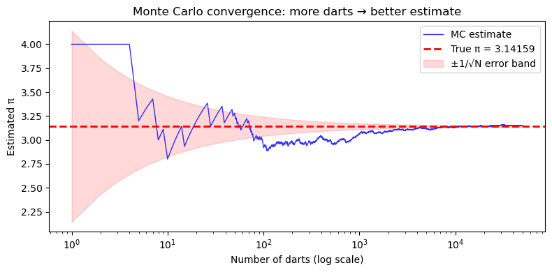
More darts = better estimate. But how fast does the estimate improve?

The key insight: the error in a Monte Carlo estimate shrinks as \(\sim 1/\sqrt{N}\).
That means to get 10× more accurate, you need 100× more samples.

This is Monte Carlo’s main limitation — it’s not very efficient for 1D problems. But it shines for high-dimensional problems (many uncertain inputs), where traditional methods become impractical.

# Throw 50,000 darts and track the running estimate of π
rng2 = np.random.default_rng(seed=0)
N_total = 50_000

x_all = rng2.random(N_total)
y_all = rng2.random(N_total)
inside_all = (x_all**2 + y_all**2) <= 1.0

# Running estimate after each dart
N_run = np.arange(1, N_total + 1)
pi_running = 4.0 * np.cumsum(inside_all) / N_run

# Plot convergence
fig, ax = plt.subplots(figsize=(8, 4))
ax.semilogx(N_run, pi_running, 'b-', linewidth=1, alpha=0.8, label='MC estimate')
ax.axhline(np.pi, color='red', linestyle='--', linewidth=2, label=f'True π = {np.pi:.5f}')
ax.fill_between(N_run, np.pi - 1/np.sqrt(N_run), np.pi + 1/np.sqrt(N_run),
                alpha=0.15, color='red', label='±1/√N error band')
ax.set_xlabel('Number of darts (log scale)')
ax.set_ylabel('Estimated π')
ax.set_title('Monte Carlo convergence: more darts → better estimate')
ax.legend()
plt.tight_layout()
plt.show()

print(f"Final estimate with {N_total:,} darts: π ≈ {pi_running[-1]:.5f}  (true: {np.pi:.5f})")

Final estimate with 50,000 darts: π ≈ 3.14968  (true: 3.14159)

14.3 A Real Engineering Problem: Process Reliability

Now let’s apply Monte Carlo to a chemical engineering scenario.

Problem statement

A chemical product must have purity ≥ 97.5% to be sold. The purity depends on two process variables that fluctuate daily due to normal operating variability:

Variable	Symbol	Distribution
Residence time (s)	\(\tau\)	\(\mathcal{N}(\mu=120,\, \sigma=12)\)
Temperature (K)	\(T\)	\(\mathcal{N}(\mu=400,\, \sigma=8)\)

The purity model is: $\( \text{Purity} = 100 \times \left(1 - 0.2\, e^{-k(T)\,\tau} \right), \quad k(T) = \exp\!\left(\frac{-1550}{T}\right) \)$

Question: What fraction of batches will fail the purity spec?

We’ll build up to the full simulation in four steps:

1. Visualize the input distributions

2. Compute purity at the mean values — and ask: is that enough information?

3. Sample a few batches by hand to see success and failure cases

4. Run the full Monte Carlo

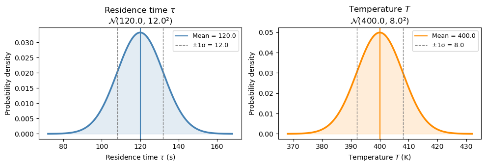
Step 1: Visualize the input distributions

Before running any simulation, let’s see what the two uncertain inputs look like. Each day, τ and T are drawn from their respective normal distributions.

import numpy as np
import matplotlib.pyplot as plt
from scipy import stats

tau_mean, tau_std = 120.0, 12.0   # residence time (s)
T_mean,   T_std   = 400.0,  8.0   # temperature (K)

fig, axes = plt.subplots(1, 2, figsize=(10, 3.5))

for ax, mean, std, label, unit, color in [
    (axes[0], tau_mean, tau_std, r'Residence time $\tau$', 's',  'steelblue'),
    (axes[1], T_mean,   T_std,   r'Temperature $T$',       'K',  'darkorange'),
]:
    x = np.linspace(mean - 4*std, mean + 4*std, 300)
    ax.plot(x, stats.norm.pdf(x, mean, std), color=color, linewidth=2.5)
    ax.fill_between(x, stats.norm.pdf(x, mean, std), alpha=0.15, color=color)
    ax.axvline(mean,       color=color,  linestyle='-',  linewidth=1.5, label=f'Mean = {mean}')
    ax.axvline(mean - std, color='gray', linestyle='--', linewidth=1,   label=f'±1σ = {std}')
    ax.axvline(mean + std, color='gray', linestyle='--', linewidth=1)
    ax.set_xlabel(f'{label} ({unit})')
    ax.set_ylabel('Probability density')
    ax.set_title(f'{label}\n' + r'$\mathcal{N}$' + f'({mean}, {std}²)')
    ax.legend(fontsize=9)

plt.tight_layout()
plt.show()

Step 2: Purity at the mean values

A natural first question: if everything runs at its mean value, what is the purity?

def purity_model(tau, T):
    k = np.exp(-1550.0 / T)
    return 100.0 * (1.0 - 0.2 * np.exp(-k * tau))

spec = 97.5   # minimum acceptable purity (%)

purity_at_mean = purity_model(tau_mean, T_mean)

print(f"At mean conditions:  τ = {tau_mean} s,  T = {T_mean} K")
print(f"  k(T_mean) = {np.exp(-1550/T_mean):.5f} s⁻¹")
print(f"  k·τ       = {np.exp(-1550/T_mean)*tau_mean:.3f}")
print(f"  Purity    = {purity_at_mean:.3f} %")
print()
if purity_at_mean >= spec:
    print(f"  Passes spec ({spec}%) at the mean — but does every batch pass?")
else:
    print(f"  Already fails spec ({spec}%) at the mean!")

At mean conditions:  τ = 120.0 s,  T = 400.0 K
  k(T_mean) = 0.02075 s⁻¹
  k·τ       = 2.491
  Purity    = 98.343 %

  Passes spec (97.5%) at the mean — but does every batch pass?

Step 3: A few sampled batches — success and failure

The mean purity looks fine. But each real batch runs at a slightly different τ and T. Let’s sample 10 batches and compute purity for each one to see how much it varies.

rng = np.random.default_rng(seed=3)
n_preview = 10

tau_s = rng.normal(tau_mean, tau_std, n_preview)
T_s   = rng.normal(T_mean,   T_std,   n_preview)
pur_s = purity_model(tau_s, T_s)

print(f"{'Batch':>5}  {'τ (s)':>8}  {'T (K)':>8}  {'Purity (%)':>11}  {'Result':>8}")
print("-" * 50)
for i in range(n_preview):
    result = "PASS ✓" if pur_s[i] >= spec else "FAIL ✗"
    print(f"  {i+1:>3}  {tau_s[i]:>8.1f}  {T_s[i]:>8.1f}  {pur_s[i]:>11.3f}  {result:>8}")

Batch     τ (s)     T (K)   Purity (%)    Result
--------------------------------------------------
    1     144.5     401.8       99.054    PASS ✓
    2      89.3     397.2       96.706    FAIL ✗
    3     125.0     397.7       98.420    PASS ✓
    4     113.2     394.7       97.847    PASS ✓
    5     114.6     391.6       97.755    PASS ✓
    6     117.4     396.9       98.118    PASS ✓
    7      95.8     403.9       97.457    FAIL ✗
    8     117.2     398.1       98.164    PASS ✓
    9     109.6     407.7       98.269    PASS ✓
   10     159.9     398.4       99.238    PASS ✓

fig, ax = plt.subplots(figsize=(5, 4))

for i in range(n_preview):
    color  = 'steelblue' if pur_s[i] >= spec else 'salmon'
    marker = 'o'         if pur_s[i] >= spec else 'X'
    label  = ('Pass ✓' if pur_s[i] >= spec else 'Fail ✗') if i == 0 or (pur_s[i] >= spec) != (pur_s[i-1] >= spec) else ''
    ax.scatter(tau_s[i], T_s[i], color=color, marker=marker, s=100, zorder=3)
    ax.annotate(f"#{i+1}: {pur_s[i]:.1f}%", (tau_s[i], T_s[i]),
                textcoords='offset points', xytext=(6, 4), fontsize=8)

# Mark the mean
ax.scatter(tau_mean, T_mean, color='black', marker='+', s=200, linewidths=2.5,
           zorder=4, label='Mean (τ, T)')

# Legend proxies
from matplotlib.lines import Line2D
handles = [
    Line2D([0],[0], marker='o', color='w', markerfacecolor='steelblue', markersize=9, label='Pass ✓'),
    Line2D([0],[0], marker='X', color='w', markerfacecolor='salmon',    markersize=9, label='Fail ✗'),
    Line2D([0],[0], marker='+', color='black', markersize=10, linewidth=2, label='Mean'),
]
ax.legend(handles=handles, fontsize=9)
ax.set_xlabel('Residence time τ (s)')
ax.set_ylabel('Temperature T (K)')
ax.set_title('10 sampled batches in (τ, T) space')
plt.tight_layout()
plt.show()

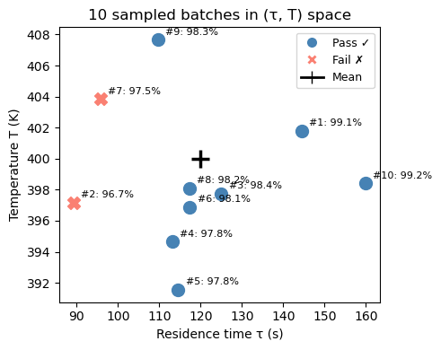
With only 10 batches we can already see some failures — but 10 is not enough to reliably estimate the failure rate. We need to scale this up to thousands of batches. That’s exactly what Monte Carlo does.

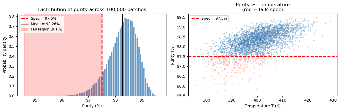
Step 4: Full Monte Carlo — 100,000 batches

rng_mc = np.random.default_rng(seed=42)
N_mc   = 100_000

# Sample all batches at once
tau_mc = rng_mc.normal(tau_mean, tau_std, N_mc)
T_mc   = rng_mc.normal(T_mean,   T_std,   N_mc)
pur_mc = purity_model(tau_mc, T_mc)

frac_fail = np.mean(pur_mc < spec)
frac_pass = 1.0 - frac_fail

print("=" * 45)
print(f"  Monte Carlo results  (N = {N_mc:,} batches)")
print("=" * 45)
print(f"  Mean purity:        {np.mean(pur_mc):.3f} %")
print(f"  Std dev:            {np.std(pur_mc, ddof=1):.3f} %")
print(f"  5th percentile:     {np.percentile(pur_mc,  5):.3f} %")
print(f"  Spec limit:         {spec} %")
print(f"  Fraction PASSING:   {frac_pass:.4f}  ({100*frac_pass:.2f}%)")
print(f"  Fraction FAILING:   {frac_fail:.4f}  ({100*frac_fail:.2f}%)")
print("=" * 45)

fig, axes = plt.subplots(1, 2, figsize=(12, 4))

# Left: purity histogram
ax = axes[0]
ax.hist(pur_mc, bins=80, density=True, color='steelblue', edgecolor='white', alpha=0.8)
ax.axvline(spec, color='red', linestyle='--', linewidth=2.5, label=f'Spec = {spec}%')
ax.axvline(np.mean(pur_mc), color='k', linestyle='-', linewidth=2,
           label=f'Mean = {np.mean(pur_mc):.2f}%')
ymax = ax.get_ylim()[1]
ax.fill_betweenx([0, ymax], pur_mc.min(), spec,
                 alpha=0.2, color='red', label=f'Fail region ({100*frac_fail:.1f}%)')
ax.set_ylim(0, ymax)
ax.set_xlabel('Purity (%)'); ax.set_ylabel('Probability density')
ax.set_title('Distribution of purity across 100,000 batches')
ax.legend(fontsize=9)

# Right: purity vs temperature scatter (subset)
ax = axes[1]
n_plot = 3000
colors = np.where(pur_mc[:n_plot] < spec, 'salmon', 'steelblue')
ax.scatter(T_mc[:n_plot], pur_mc[:n_plot], c=colors, alpha=0.3, s=5)
ax.axhline(spec, color='red', linestyle='--', linewidth=2, label=f'Spec = {spec}%')
ax.set_xlabel('Temperature T (K)'); ax.set_ylabel('Purity (%)')
ax.set_title('Purity vs. Temperature\n(red = fails spec)')
ax.legend(fontsize=9)

plt.tight_layout()
plt.show()

=============================================
  Monte Carlo results  (N = 100,000 batches)
=============================================
  Mean purity:        98.265 %
  Std dev:            0.546 %
  5th percentile:     97.264 %
  Spec limit:         97.5 %
  Fraction PASSING:   0.9089  (90.89%)
  Fraction FAILING:   0.0911  (9.11%)
=============================================

What did we learn from this simulation?

• The mean purity (~98.3%) is above the spec, which might make you think the process is fine.

• But the output distribution has a spread of ~0.5–0.7%, so the tail dips below 97.5%.

• Monte Carlo tells us roughly ~9% of batches will fail — a number you cannot get from just computing purity at the mean.

• The scatter plot shows failures cluster at lower temperatures and shorter residence times — both reduce the rate constant and slow the reaction.

This is the central lesson: the mean alone is not enough. You need the full distribution.

---

14.4 Summary

Concept	Key idea
Monte Carlo simulation	Estimate outputs by sampling inputs randomly and running the model many times
Random number generator	rng = np.random.default_rng(seed=...) creates reproducible random numbers
Sampling from a distribution	rng.normal(mean, std, N) for normal; rng.uniform(low, high, N) for uniform
Output analysis	Use np.mean(), np.std(), np.percentile() on the output array
Convergence	Error shrinks as \(\sim 1/\sqrt{N}\) — more samples = more accurate

The Monte Carlo template (reuse this!)

import numpy as np

rng = np.random.default_rng(seed=42)
N = 100_000

# 1. Sample inputs
x1 = rng.normal(mean1, std1, N)
x2 = rng.normal(mean2, std2, N)

# 2. Compute output for all samples at once
output = my_model(x1, x2)   # works if my_model uses numpy operations

# 3. Summarize
print(f"Mean:   {np.mean(output):.3f}")
print(f"Std:    {np.std(output):.3f}")
print(f"P(output < threshold) = {np.mean(output < threshold):.4f}")