Chapter 12: Polynomial Fitting & Interpolation

Topics Covered:

• Polynomial basics: np.poly1d, np.polyval, np.polyfit

• Least-squares polynomial fitting: choosing the right degree, residuals, \(R^2\)

• Taylor series: definition, convergence, and ChE linearization

• Polynomial interpolation: Lagrange method and Runge’s phenomenon

• Spline interpolation: CubicSpline, interp1d, and steam table application

# ── All imports ─────────────────────────────────────────────────────────────
import numpy as np
import matplotlib.pyplot as plt

12.1 Motivation: Heat Capacity of CO\(_2\)

In chemical engineering, we frequently need \(C_p(T)\) — the molar heat capacity as a function of temperature — to compute:

\[ Q = n \int_{T_1}^{T_2} C_p(T)\, dT \]

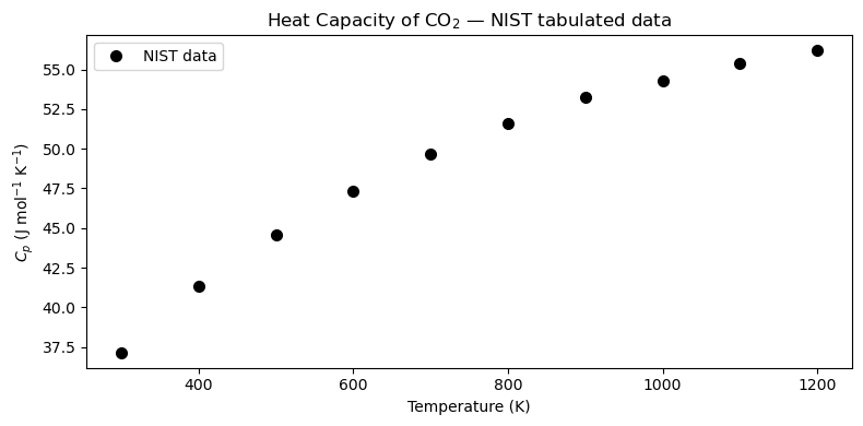
NIST publishes \(C_p\) in tabulated form at discrete temperatures. Before we can integrate, we need a continuous mathematical model — a polynomial — that passes smoothly through the data.

Below is a subset of NIST data for CO\(_2\) (ideal gas, J mol\(^{-1}\) K\(^{-1}\)):

\(T\) (K)	\(C_p\) (J mol\(^{-1}\) K\(^{-1}\))
300	37.13
400	41.33
500	44.60
600	47.33
700	49.65
800	51.61
900	53.26
1000	54.31
1100	55.37
1200	56.21

We want to fit \(C_p(T) \approx a_0 + a_1 T + a_2 T^2 + \cdots\) so we can evaluate it at any temperature and integrate it analytically.

# NIST tabulated Cp data for CO2 (ideal gas)
T_data  = np.array([300, 400, 500, 600, 700, 800, 900, 1000, 1100, 1200], dtype=float)  # K
Cp_data = np.array([37.13, 41.33, 44.60, 47.33, 49.65,
                    51.61, 53.26, 54.31, 55.37, 56.21])  # J/(mol K)

fig, ax = plt.subplots(figsize=(8, 4))
ax.plot(T_data, Cp_data, 'ko', markersize=7, label='NIST data')
ax.set_xlabel('Temperature (K)')
ax.set_ylabel(r'$C_p$ (J mol$^{-1}$ K$^{-1}$)')
ax.set_title(r'Heat Capacity of CO$_2$ — NIST tabulated data')
ax.legend()
plt.tight_layout()
plt.show()

12.2 Polynomial Basics

A degree-\(n\) polynomial is:

\[ p(x) = a_n x^n + a_{n-1} x^{n-1} + \cdots + a_1 x + a_0 \]

NumPy stores polynomial coefficients in descending order (highest power first). Three key tools:

Function	Purpose
np.poly1d(coeffs)	Create a callable polynomial object
np.polyval(coeffs, x)	Evaluate polynomial at \(x\)
np.polyfit(x, y, deg)	Least-squares fit: returns coefficients

Convention: coeffs = [a_n, a_{n-1}, ..., a_1, a_0] — highest power first.

---

The coefficient array

Say you have \(p(x) = 3x^2 + 5x - 2\). NumPy represents this as [3, 5, -2]:

index:  0    1    2
value: [3,   5,  -2]
         ↑    ↑    ↑
        x²   x¹   x⁰

np.poly1d(coeffs) — callable polynomial object

Wraps the coefficient list into an object you can call like a function:

p = np.poly1d([3, 5, -2])
p(1)   # → 3(1)² + 5(1) - 2 = 6
p(0)   # → -2

Bonus methods: p.deriv() (derivative), p.integ() (integral), p.roots (zeros).

np.polyval(coeffs, x) — evaluate from the list directly

Same result, no object needed. Works on scalars or arrays:

np.polyval([3, 5, -2], 1)           # → 6
np.polyval([3, 5, -2], [0, 1, 2])   # → [-2, 6, 20]

Use this when you only need values and don’t need derivatives/integrals.

np.polyfit(x, y, deg) — find best-fit coefficients

Given data points, returns a coefficient array in the same descending convention:

coeffs = np.polyfit(x_data, y_data, deg=3)  # fit  → coeffs
p      = np.poly1d(coeffs)                  # wrap → callable
y_fit  = p(x_fine)                          # evaluate on dense grid
# or equivalently:
y_fit  = np.polyval(coeffs, x_fine)

Use poly1d when you also need .deriv() / .integ() / .roots; use polyval when you just need numbers.

# ── Coefficient convention demo ───────────────────────────────────────────
# p(x) = 3x² + 5x - 2   →   coeffs = [3, 5, -2]  (descending order)
coeffs_demo = [3, 5, -2]

p_demo = np.poly1d(coeffs_demo)
print("poly1d pretty-print:")
print(p_demo)

# Evaluate at a few points
xs = [0, 1, 2]
print("\nx   poly1d   polyval   manual")
for x in xs:
    manual = 3*x**2 + 5*x - 2
    print(f"{x}   {p_demo(x):6.1f}   {np.polyval(coeffs_demo, x):6.1f}   {manual:6.1f}")

# polyval works on arrays too
print("\npolyval on array [0,1,2]:", np.polyval(coeffs_demo, xs))

# Derivative and integral via poly1d
print("\nDerivative p'(x):")
print(p_demo.deriv())
print("Indefinite integral ∫p dx (+ C):")
print(p_demo.integ())
print("Roots (p(x)=0):", p_demo.roots.round(4))

poly1d pretty-print:
   2
3 x + 5 x - 2

x   poly1d   polyval   manual
0     -2.0     -2.0     -2.0
1      6.0      6.0      6.0
2     20.0     20.0     20.0

polyval on array [0,1,2]: [-2  6 20]

Derivative p'(x):
 
6 x + 5
Indefinite integral ∫p dx (+ C):
   3       2
1 x + 2.5 x - 2 x
Roots (p(x)=0): [-2.      0.3333]

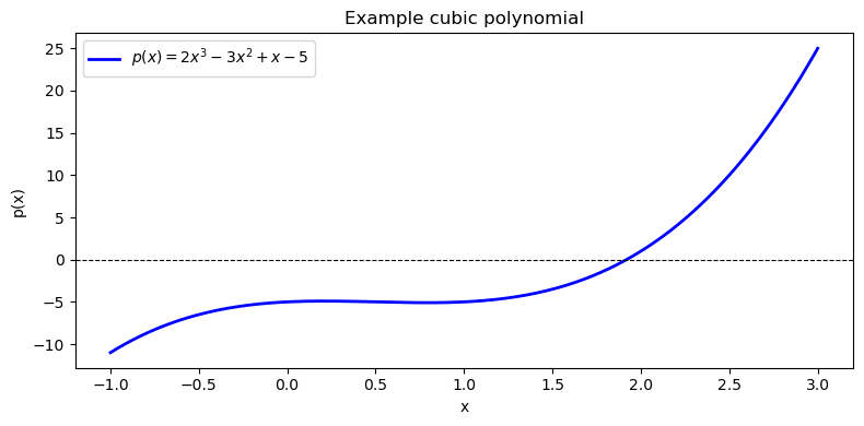
# Define p(x) = 2x^3 - 3x^2 + x - 5  (coefficients in descending order)
coeffs = [2, -3, 1, -5]

p = np.poly1d(coeffs)
print("Polynomial p(x):")
print(p)

# Evaluate at x = 2
x_val = 2.0
print(f"\np({x_val}) using poly1d  : {p(x_val):.4f}")
print(f"p({x_val}) using polyval : {np.polyval(coeffs, x_val):.4f}")
# Manual: 2(8) - 3(4) + 1(2) - 5 = 16 - 12 + 2 - 5 = 1
print(f"Manual check          : {2*x_val**3 - 3*x_val**2 + 1*x_val - 5:.4f}")

Polynomial p(x):
   3     2
2 x - 3 x + 1 x - 5

p(2.0) using poly1d  : 1.0000
p(2.0) using polyval : 1.0000
Manual check          : 1.0000

# Plot the polynomial over [-1, 3]
x = np.linspace(-1, 3, 200)
y = np.polyval(coeffs, x)

fig, ax = plt.subplots(figsize=(8, 4))
ax.plot(x, y, 'b-', linewidth=2, label=r'$p(x) = 2x^3 - 3x^2 + x - 5$')
ax.axhline(0, color='k', linewidth=0.8, linestyle='--')
ax.set_xlabel('x')
ax.set_ylabel('p(x)')
ax.set_title('Example cubic polynomial')
ax.legend()
plt.tight_layout()
plt.show()

12.3 Least-Squares Polynomial Fitting

np.polyfit(x, y, deg) finds the degree-deg polynomial coefficients that minimize the sum of squared residuals:

\[ \min_{a_0, \ldots, a_n} \sum_{i=1}^{N} \left[ y_i - p(x_i) \right]^2 \]

This is ordinary least squares applied to a polynomial basis. The function returns coefficients in descending order (highest power first), just like np.poly1d expects.

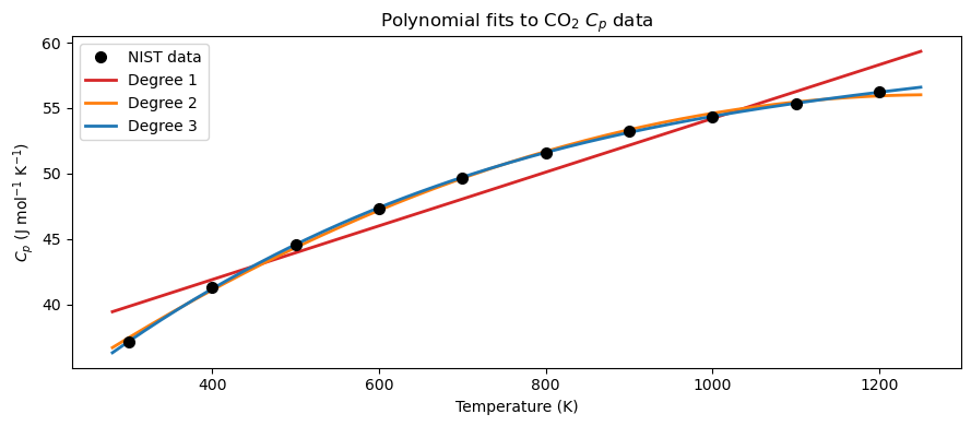
12.3.1 Fitting Cp(T) with Different Degrees

We fit the CO\(_2\) data with degree 1, 2, and 3 polynomials and compare the results visually.

# ── Fit Cp(T) with degree 1, 2, 3 polynomials ────────────────────────────────
T_fine  = np.linspace(280, 1250, 300)
degrees = [1, 2, 3]
colors  = ['tab:red', 'tab:orange', 'tab:blue']
fits    = {}    # store coefficient arrays keyed by degree

for deg in degrees:
    fits[deg] = np.polyfit(T_data, Cp_data, deg)

fig, ax = plt.subplots(figsize=(9, 4))
ax.plot(T_data, Cp_data, 'ko', markersize=7, zorder=5, label='NIST data')
for deg, color in zip(degrees, colors):
    ax.plot(T_fine, np.polyval(fits[deg], T_fine),
            color=color, linewidth=2, label=f'Degree {deg}')
ax.set_xlabel('Temperature (K)')
ax.set_ylabel(r'$C_p$ (J mol$^{-1}$ K$^{-1}$)')
ax.set_title(r'Polynomial fits to CO$_2$ $C_p$ data')
ax.legend()
plt.tight_layout()
plt.show()

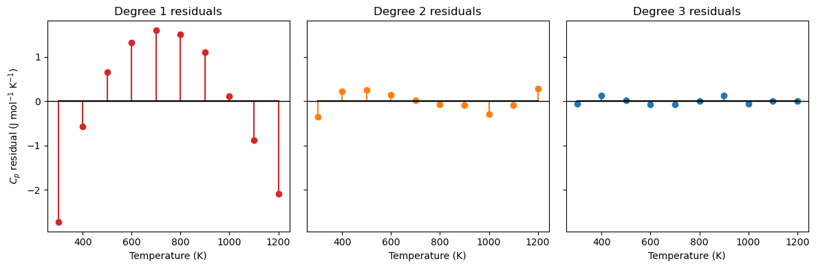
The residual \(e_i\) is the vertical distance between a measured data point and the model’s prediction at that same \(x\):

\[ e_i = y_i - p(x_i) \]

A positive residual means the model underpredicts; negative means it overpredicts. A good fit has residuals that are small and scattered randomly around zero.

# ── Residual stem plots for each degree ──────────────────────────────────────
fig, axes = plt.subplots(1, 3, figsize=(12, 4), sharey=True)

for ax, deg, color in zip(axes, degrees, colors):
    Cp_pred   = np.polyval(fits[deg], T_data)
    residuals = Cp_data - Cp_pred
    ax.stem(T_data, residuals, linefmt=color, markerfmt='o', basefmt='k-')
    ax.axhline(0, color='k', linewidth=1)
    ax.set_xlabel('Temperature (K)')
    ax.set_title(f'Degree {deg} residuals')

axes[0].set_ylabel(r'$C_p$ residual (J mol$^{-1}$ K$^{-1}$)')
plt.tight_layout()
plt.show()

12.3.2 Fit Quality Metrics: MAE, MSE, and \(R^2\)

Given residuals \(e_i = y_i - p(x_i)\), where:

• \(y_i\) — observed (measured) value at point \(i\)

• \(p(x_i)\) — model-predicted value at the same point \(x_i\)

three standard metrics quantify how well the model fits the data:

\[ \text{MAE} = \frac{1}{N}\sum_{i=1}^{N} |e_i| \qquad \text{MSE} = \frac{1}{N}\sum_{i=1}^{N} e_i^2 \qquad R^2 = 1 - \frac{\sum_i e_i^2}{\sum_i (y_i - \bar{y})^2} \]

Metric	Full name	Units	Interpretation
MAE	Mean Absolute Error	same as \(y\)	Average magnitude of error; easy to interpret
MSE	Mean Squared Error	\(y^2\)	Penalizes large errors more heavily; used by least-squares optimization
\(R^2\)	Coefficient of Determination	dimensionless	Fraction of variance explained by the model; 1 = perfect

Why square in MSE (and not just use MAE)?

• Penalize large errors more heavily — an error of 2 contributes 4× more than an error of 1; the fit is driven by the worst offenders

• Smooth, differentiable objective — \(e_i^2\) has a clean derivative everywhere, which is what allows least-squares to be solved analytically; \(|e_i|\) is not differentiable at zero

Interpreting \(R^2\): The denominator \(\sum_i(y_i - \bar{y})^2\) is the total variance in the data (how spread out the measurements are). The numerator \(\sum_i e_i^2\) is the variance the model failed to explain. Subtracting their ratio from 1 gives the fraction the model does explain.

• \(R^2 = 1\) — perfect fit; every residual is zero

• \(R^2 = 0\) — the model does no better than just predicting \(\bar{y}\) for every point

• \(R^2 < 0\) — the model is worse than the mean (a sign something is seriously wrong)

import numpy as np
# ── MAE, MSE, R² for each polynomial degree ──────────────────────────────────
SS_tot = np.sum((Cp_data - np.mean(Cp_data))**2)

print(f"{'Degree':>6}  {'MAE':>18}  {'MSE':>18}  {'R²':>10}")
print(f"{'':>6}  {'(J/mol/K)':>18}  {'(J/mol/K)²':>18}  {'':>10}")
print("-" * 60)
for deg in degrees:
    Cp_pred   = np.polyval(fits[deg], T_data)
    residuals = Cp_data - Cp_pred
    MAE = np.mean(np.abs(residuals))
    MSE = np.mean(residuals**2)
    R2  = 1.0 - np.sum(residuals**2) / SS_tot
    print(f"{deg:>6}  {MAE:>18.6f}  {MSE:>18.6f}  {R2:>10.6f}")

Degree                 MAE                 MSE          R²
                 (J/mol/K)          (J/mol/K)²            
------------------------------------------------------------
     1            1.256000            2.114124    0.942543
     2            0.179212            0.043519    0.998817
     3            0.052923            0.004851    0.999868

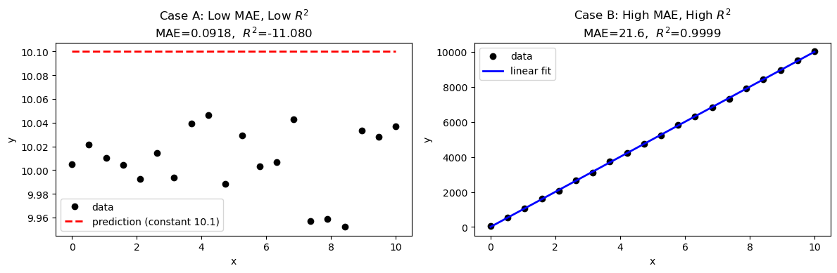
12.3.3 MAE vs \(R^2\): They Can Disagree

MAE and \(R^2\) measure different things, so a model can score well on one and poorly on the other.

Case A — Low MAE, low \(R^2\): All errors are small in absolute magnitude, but the data has almost no variance. The model barely outperforms the flat mean, so \(R^2\) stays near zero even though MAE looks fine.

Case B — High MAE, high \(R^2\): The data has a huge range (high variance). Errors are large in absolute units, giving a high MAE — but the model tracks the trend so well that \(R^2\) is still close to 1.

The takeaway: always report both. MAE tells you the error in physical units (is it acceptable for your application?); \(R^2\) tells you whether the model captures the structure of the data.

import numpy as np
import matplotlib.pyplot as plt

def metrics(y, y_pred):
    e    = y - y_pred
    mae  = np.mean(np.abs(e))
    mse  = np.mean(e**2)
    ss_res = np.sum(e**2)
    ss_tot = np.sum((y - np.mean(y))**2)
    r2   = 1 - ss_res / ss_tot
    return mae, mse, r2

# ── Case A: Low MAE, Low R² ───────────────────────────────────────────────────
# Data clusters tightly around 10.0 (very low variance).
# The model predicts a constant 10.1 — errors are tiny, but so is the spread,
# so R² is low because the model barely beats the mean.
np.random.seed(0)
x_A  = np.linspace(0, 10, 20)
y_A  = 10.0 + np.random.uniform(-0.05, 0.05, 20)   # near-flat data, range ≈ 0.1
yp_A = np.full_like(y_A, 10.1)                     # constant prediction slightly off

mae_A, mse_A, r2_A = metrics(y_A, yp_A)
print("Case A — Low MAE, Low R²")
print(f"  Data range : {y_A.min():.3f} – {y_A.max():.3f}  (spread ≈ {y_A.max()-y_A.min():.3f})")
print(f"  MAE = {mae_A:.4f}    MSE = {mse_A:.6f}    R² = {r2_A:.4f}")

# ── Case B: High MAE, High R² ─────────────────────────────────────────────────
# Data spans 0–10 000 (huge variance) with a clean linear trend.
# A linear fit tracks it perfectly (R² ≈ 1), but residuals are ~50 units → high MAE.
x_B  = np.linspace(0, 10, 20)
y_B  = 1000 * x_B + np.random.uniform(-50, 50, 20)   # large range, noisy
coeffs_B = np.polyfit(x_B, y_B, 1)
yp_B = np.polyval(coeffs_B, x_B)

mae_B, mse_B, r2_B = metrics(y_B, yp_B)
print("\nCase B — High MAE, High R²")
print(f"  Data range : {y_B.min():.1f} – {y_B.max():.1f}  (spread ≈ {y_B.max()-y_B.min():.1f})")
print(f"  MAE = {mae_B:.4f}    MSE = {mse_B:.2f}    R² = {r2_B:.4f}")

# ── Plot ──────────────────────────────────────────────────────────────────────
fig, axes = plt.subplots(1, 2, figsize=(12, 4))

ax = axes[0]
ax.plot(x_A, y_A,  'ko', markersize=6, label='data')
ax.plot(x_A, yp_A, 'r--', linewidth=2, label='prediction (constant 10.1)')
ax.set_title(f'Case A: Low MAE, Low $R^2$\nMAE={mae_A:.4f},  $R^2$={r2_A:.3f}')
ax.set_xlabel('x'); ax.set_ylabel('y')
ax.legend()

ax = axes[1]
ax.plot(x_B, y_B,  'ko', markersize=6, label='data')
ax.plot(x_B, yp_B, 'b-', linewidth=2, label='linear fit')
ax.set_title(f'Case B: High MAE, High $R^2$\nMAE={mae_B:.1f},  $R^2$={r2_B:.4f}')
ax.set_xlabel('x'); ax.set_ylabel('y')
ax.legend()

plt.tight_layout()
plt.show()

Case A — Low MAE, Low R²
  Data range : 9.952 – 10.046  (spread ≈ 0.094)
  MAE = 0.0918    MSE = 0.009197    R² = -11.0804

Case B — High MAE, High R²
  Data range : 47.9 – 10018.2  (spread ≈ 9970.3)
  MAE = 21.6016    MSE = 721.01    R² = 0.9999

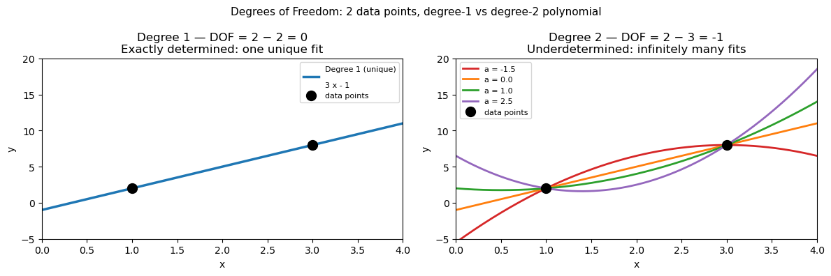
12.3.4 Degrees of Freedom in Polynomial Fitting

Degrees of freedom (DOF) quantify how much “slack” a model has after satisfying all data constraints:

\[\text{DOF} = N - p\]

where \(N\) = number of data points and \(p\) = number of model parameters (coefficients).

---

1. Linear fit (degree 1)

\[y = ax + b \qquad (p = 2 \text{ parameters})\]

With \(N = 2\) data points:

\[\text{DOF} = 2 - 2 = 0\]

DOF = 0 means the system is exactly determined — one unique line passes through both points, with zero residuals by construction.

---

2. Quadratic fit (degree 2)

\[y = ax^2 + bx + c \qquad (p = 3 \text{ parameters})\]

With \(N = 2\) data points:

\[\text{DOF} = 2 - 3 = -1\]

DOF < 0 means the system is underdetermined — more parameters than constraints, so infinitely many quadratic curves pass through those two points. The fit is not unique.

---

General rule

DOF	Condition	Meaning
\(> 0\)	\(N > p\)	Overdetermined — least-squares finds the best compromise
\(= 0\)	\(N = p\)	Exactly determined — perfect interpolation, unique solution
\(< 0\)	\(N < p\)	Underdetermined — infinitely many solutions

For polynomial fitting of physical data, you almost always want DOF \(\gg 0\): many more data points than coefficients. This is what makes the fit statistically meaningful — the polynomial is constrained by real data, not just solving a system of equations.

import numpy as np
import matplotlib.pyplot as plt

# Two data points
x_pts = np.array([1.0, 3.0])
y_pts = np.array([2.0, 8.0])

x_fine = np.linspace(0, 4, 200)

# ── Degree 1: DOF = 2 - 2 = 0  (unique solution) ─────────────────────────────
c1 = np.polyfit(x_pts, y_pts, 1)       # one unique line
y1 = np.polyval(c1, x_fine)

# ── Degree 2: DOF = 2 - 3 = -1 (underdetermined — infinitely many solutions) ─
# np.polyfit returns ONE solution (minimum-norm), but infinitely many exist.
# We generate three more by varying the free parameter 'a' manually.
#   y = a*x^2 + bx + c  — with 2 equations and 3 unknowns,
#   'a' is free. Fix a, then solve for b and c.
def quadratic_through_two_points(x_pts, y_pts, a):
    """Given 'a', find b,c so that ax^2 + bx + c passes through both points."""
    x1, x2 = x_pts
    y1, y2 = y_pts
    # y1 = a*x1^2 + b*x1 + c  →  b*x1 + c = y1 - a*x1^2
    # y2 = a*x2^2 + b*x2 + c  →  b*x2 + c = y2 - a*x2^2
    A = np.array([[x1, 1], [x2, 1]])
    rhs = np.array([y1 - a*x1**2, y2 - a*x2**2])
    b, c = np.linalg.solve(A, rhs)
    return np.array([a, b, c])

a_values = [-1.5, 0.0, 1.0, 2.5]   # four choices of the free parameter
colors_q  = ['tab:red', 'tab:orange', 'tab:green', 'tab:purple']

fig, axes = plt.subplots(1, 2, figsize=(12, 4))

# Left: degree 1 (unique)
ax = axes[0]
ax.plot(x_fine, y1, 'tab:blue', linewidth=2.5, label=f'Degree 1 (unique)\n{np.poly1d(c1)}')
ax.plot(x_pts, y_pts, 'ko', markersize=10, zorder=5, label='data points')
ax.set_title(f'Degree 1 — DOF = {len(x_pts)} − 2 = {len(x_pts)-2}\nExactly determined: one unique fit')
ax.set_xlabel('x'); ax.set_ylabel('y')
ax.set_xlim(0, 4); ax.set_ylim(-5, 20)
ax.legend(fontsize=8)

# Right: degree 2 (infinitely many)
ax = axes[1]
for a_val, col in zip(a_values, colors_q):
    coeffs_q = quadratic_through_two_points(x_pts, y_pts, a_val)
    ax.plot(x_fine, np.polyval(coeffs_q, x_fine), color=col,
            linewidth=2, label=f'a = {a_val}')
ax.plot(x_pts, y_pts, 'ko', markersize=10, zorder=5, label='data points')
ax.set_title(f'Degree 2 — DOF = {len(x_pts)} − 3 = {len(x_pts)-3}\nUnderdetermined: infinitely many fits')
ax.set_xlabel('x'); ax.set_ylabel('y')
ax.set_xlim(0, 4); ax.set_ylim(-5, 20)
ax.legend(fontsize=8)

plt.suptitle('Degrees of Freedom: 2 data points, degree-1 vs degree-2 polynomial', fontsize=11)
plt.tight_layout()
plt.show()

print("Degree 1 (DOF = 0):")
print(f"  Unique coefficients: {c1.round(4)}")
print()
print("Degree 2 (DOF = -1) — all four pass exactly through the same two points:")
for a_val in a_values:
    c = quadratic_through_two_points(x_pts, y_pts, a_val)
    print(f"  a={a_val:+.1f} → coeffs = {c.round(4)}  | check: p({x_pts[0]})={np.polyval(c, x_pts[0]):.1f}, p({x_pts[1]})={np.polyval(c, x_pts[1]):.1f}")

Degree 1 (DOF = 0):
  Unique coefficients: [ 3. -1.]

Degree 2 (DOF = -1) — all four pass exactly through the same two points:
  a=-1.5 → coeffs = [-1.5  9.  -5.5]  | check: p(1.0)=2.0, p(3.0)=8.0
  a=+0.0 → coeffs = [ 0.  3. -1.]  | check: p(1.0)=2.0, p(3.0)=8.0
  a=+1.0 → coeffs = [ 1. -1.  2.]  | check: p(1.0)=2.0, p(3.0)=8.0
  a=+2.5 → coeffs = [ 2.5 -7.   6.5]  | check: p(1.0)=2.0, p(3.0)=8.0

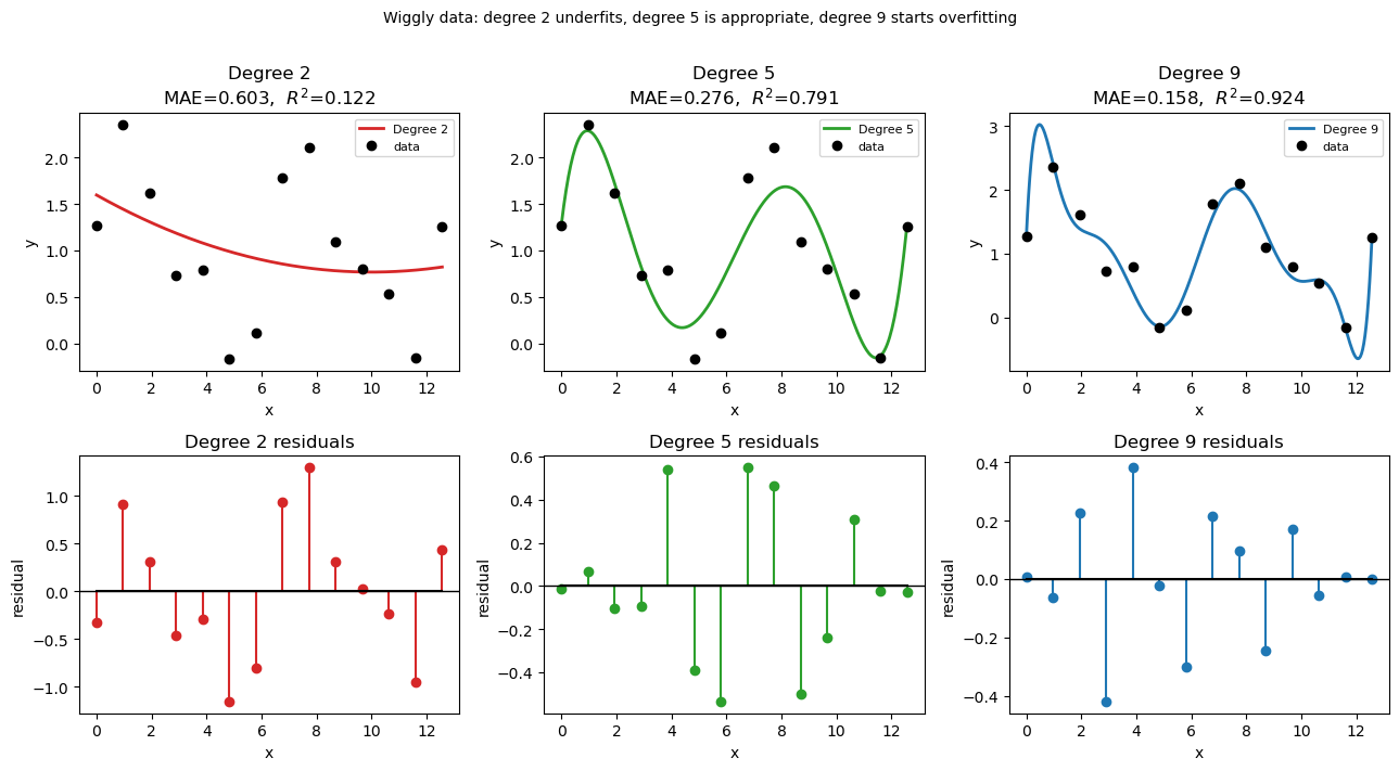
12.3.5 Overfitting: When Higher Degree Hurts

Adding more polynomial terms always reduces training error, but can create overfitting: the polynomial wiggles between data points and performs poorly outside the training range.

Why does adding terms always reduce training error? With \(N\) data points and a degree-\((N-1)\) polynomial, you have exactly enough free coefficients to pass through every point perfectly — residuals become zero by construction. But this is not a good model; it has memorized the noise in the data rather than learned the underlying trend.

Degrees of freedom = number of adjustable parameters (coefficients) available to fit the data. A degree-\(n\) polynomial has \(n+1\) coefficients, so \(n+1\) degrees of freedom.

Degree	Degrees of freedom	Behavior
High (\(N-1\))	\(N\) — one per data point	Zero training error · High variance · Overfitting risk
Low–moderate	\(\ll N\)	Nonzero residual · Better generalization · Controlled flexibility

The bias-variance tradeoff:

• A low-degree polynomial is too rigid — it misses real structure in the data

• A high-degree polynomial is too flexible — it chases every fluctuation and noise spike

The right degree sits in between: flexible enough to capture the physical trend, not so flexible that it fits the noise. A practical warning sign: if the polynomial behaves wildly between data points or shoots off just outside the data range, the degree is too high.

\[ \text{If } \deg(p) = N - 1 \text{ and you have } N \text{ points} \implies \text{SS}_{\text{res}} = 0,\quad R^2 = 1 \quad \text{(but the model is useless)} \]

Here we deliberately use degree 9 (with only 10 data points) to illustrate the problem.

import numpy as np
import matplotlib.pyplot as plt

# ── Wiggly dataset: a signal with genuine oscillations + small noise ──────────
# Imagine a periodic reaction yield measured across 12 experimental conditions.
np.random.seed(3)
x_wig = np.linspace(0, 4 * np.pi, 14)
y_wig = np.sin(x_wig) + 0.5 * np.sin(2 * x_wig) + np.random.normal(1, 0.15, 14) # np.sin(x_wig) + 0.5 * np.sin(2 * x_wig) + 


x_fine = np.linspace(0, 4 * np.pi, 300)

# Fit with degree 2, 5, and 9
degs   = [2, 5, 9]
colors = ['tab:red', 'tab:green', 'tab:blue']
fits_w = {d: np.polyfit(x_wig, y_wig, d) for d in degs}

# ── Metrics ───────────────────────────────────────────────────────────────────
SS_tot_w = np.sum((y_wig - np.mean(y_wig))**2)
print(f"{'Degree':>6}  {'MAE':>10}  {'R²':>8}  {'Note'}")
print("-" * 48)
notes = {2: 'underfit — misses oscillations',
         5: 'good fit — captures structure',
         9: 'starts to overfit noise'}
for d in degs:
    pred = np.polyval(fits_w[d], x_wig)
    res  = y_wig - pred
    mae  = np.mean(np.abs(res))
    r2   = 1 - np.sum(res**2) / SS_tot_w
    print(f"{d:>6}  {mae:>10.4f}  {r2:>8.4f}  {notes[d]}")

# ── Plot: fits ────────────────────────────────────────────────────────────────
fig, axes = plt.subplots(2, 3, figsize=(13, 7))

for col, (d, color) in enumerate(zip(degs, colors)):
    y_pred_fine = np.polyval(fits_w[d], x_fine)
    y_pred_data = np.polyval(fits_w[d], x_wig)
    residuals   = y_wig - y_pred_data
    mae  = np.mean(np.abs(residuals))
    r2   = 1 - np.sum(residuals**2) / SS_tot_w

    # Top row: fit vs data
    ax = axes[0, col]
    ax.plot(x_fine, y_pred_fine, color=color, linewidth=2, label=f'Degree {d}')
    ax.plot(x_wig, y_wig, 'ko', markersize=6, zorder=5, label='data')
    ax.set_title(f'Degree {d}\nMAE={mae:.3f},  $R^2$={r2:.3f}')
    ax.set_xlabel('x'); ax.set_ylabel('y')
    ax.legend(fontsize=8)

    # Bottom row: residuals
    ax = axes[1, col]
    ax.stem(x_wig, residuals, linefmt=color, markerfmt='o', basefmt='k-')
    ax.axhline(0, color='k', linewidth=1)
    ax.set_title(f'Degree {d} residuals')
    ax.set_xlabel('x'); ax.set_ylabel('residual')

plt.suptitle('Wiggly data: degree 2 underfits, degree 5 is appropriate, degree 9 starts overfitting',
             fontsize=10, y=1.01)
plt.tight_layout()
plt.show()

Degree         MAE        R²  Note
------------------------------------------------
     2      0.6030    0.1219  underfit — misses oscillations
     5      0.2763    0.7914  good fit — captures structure
     9      0.1583    0.9236  starts to overfit noise

# ── Overfitting demonstration ─────────────────────────────────────────────────
coeffs_deg3 = np.polyfit(T_data, Cp_data, 3)
coeffs_deg9 = np.polyfit(T_data, Cp_data, 9)

T_ext = np.linspace(200, 1300, 400)   # extend beyond the data range

fig, ax = plt.subplots(figsize=(9, 4))
ax.plot(T_data, Cp_data, 'ko', markersize=7, zorder=5, label='NIST data')
ax.plot(T_ext, np.polyval(coeffs_deg3, T_ext),
        'tab:blue', linewidth=2, label='Degree 3 (good fit)')
ax.plot(T_ext, np.polyval(coeffs_deg9, T_ext),
        'tab:red',  linewidth=2, linestyle='--', label='Degree 9 (overfit)')
ax.set_ylim(30, 80)
ax.set_xlabel('Temperature (K)')
ax.set_ylabel(r'$C_p$ (J mol$^{-1}$ K$^{-1}$)')
ax.set_title('Overfitting: degree-9 polynomial fits training data perfectly but extrapolates badly')
ax.legend()
plt.tight_layout()
plt.show()

print("Lesson: For smooth physical data, a low-degree polynomial (2-4) is usually best.")
print("Use R² and visual inspection — not just training error — to choose degree.")

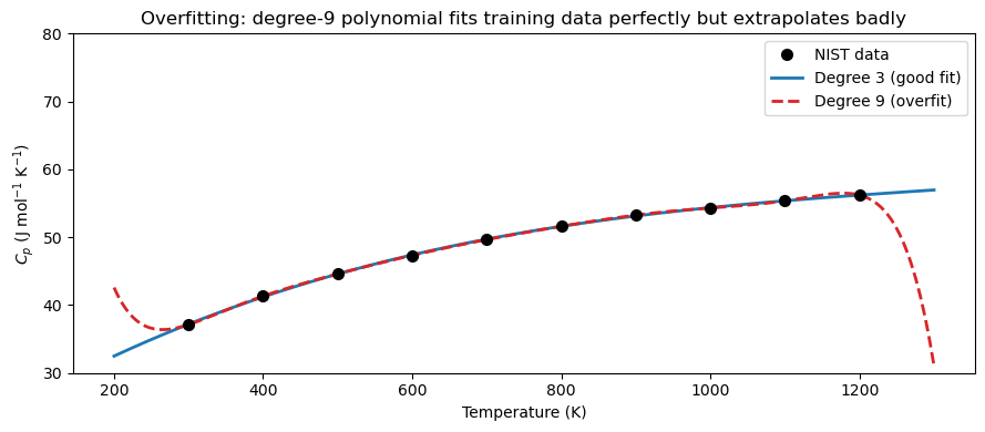
Lesson: For smooth physical data, a low-degree polynomial (2-4) is usually best.
Use R² and visual inspection — not just training error — to choose degree.

12.4 Summary

Concept	Tool / Formula	When to use
Polynomial evaluation	np.polyval(coeffs, x)	Evaluate a stored coefficient array at \(x\)
Polynomial object	np.poly1d(coeffs)	Callable; .integ() returns antiderivative
Least-squares fit	np.polyfit(x, y, deg)	Fit noisy or tabulated data; keep degree small
Residuals	\(e_i = y_i - p(x_i)\)	Signed error at each data point
MAE	\(\frac{1}{N}\sum|e_i|\)	Average error in original units; easy to interpret
MSE	\(\frac{1}{N}\sum e_i^2\)	Penalizes large errors; units are \(y^2\)
\(R^2\)	\(1 - \sum e_i^2 / \sum(y_i-\bar{y})^2\)	Fraction of variance explained; 1 = perfect