Chapter 0: Introduction to Python & Jupyter Notebooks#
0.1 Python#
Python is one of the most widely used programming languages and runs on all major operating systems, including macOS, Linux, and Windows. As free, open-source software maintained by the Python Software Foundation. Python offers two key major advantages. First, it is universally accessible—anyone can download and use it at no cost, regardless of budget. Second, because it is open source, its underlying code is publicly available for inspection and modification. This transparency allows users and developers to verify how the software works, rather than relying solely on claims made by its distributors.
0.2 Jupyter Notebooks#
Jupyter notebooks are an interactive computing environment widely used in science, engineering, and data analysis. Instead of writing code in a traditional script, a notebook is organized into cells that you can run independently. This lets you write code, see the output immediately, adjust your analysis, and document your reasoning—all in one place. Jupyter notebooks are particularly well suited for interactive coding and step-by-step demonstrations, similar to working through examples in a classroom setting.
This chapter uses Python together with Jupyter notebooks, which provide an interactive environment ideal for scientific computing. We will also work with several free, open-source libraries that expand Python’s capabilities for data processing, numerical analysis, and visualization.
0.3 Getting Started: Accessing Python and Jupyter#
To begin working with Python in this course, you will need access to three things:
Python
Jupyter Notebooks
Scientific libraries (NumPy, Pandas, Matplotlib, etc.)
There are two recommended ways to set up this environment.
Choose ONE option (you can switch later if you want).
Two Setup Options
Option 1 — Install Everything on Your Computer (Anaconda/Miniconda)
Usually faster for most tasks
Works without internet
No login or registration needed
Can open many notebooks at once
Option 2 — Use Google Colab (No Installation Needed)
No software installation required
Uses Google’s computing power, not yours
Easy real-time collaboration
Both options work with the exact same .ipynb notebook files.
For this course, we will primarily use a local conda environment. Option 2 is provided only as an alternative for students who are unable to install the software locally.
Also, JupyterLab will be used as the primary coding environment. All in-class demonstrations and course materials are based on Jupyter notebooks, which allow you to write and run code interactively, view results immediately, and combine code, equations, and explanations in one place—similar to working through problems in class.
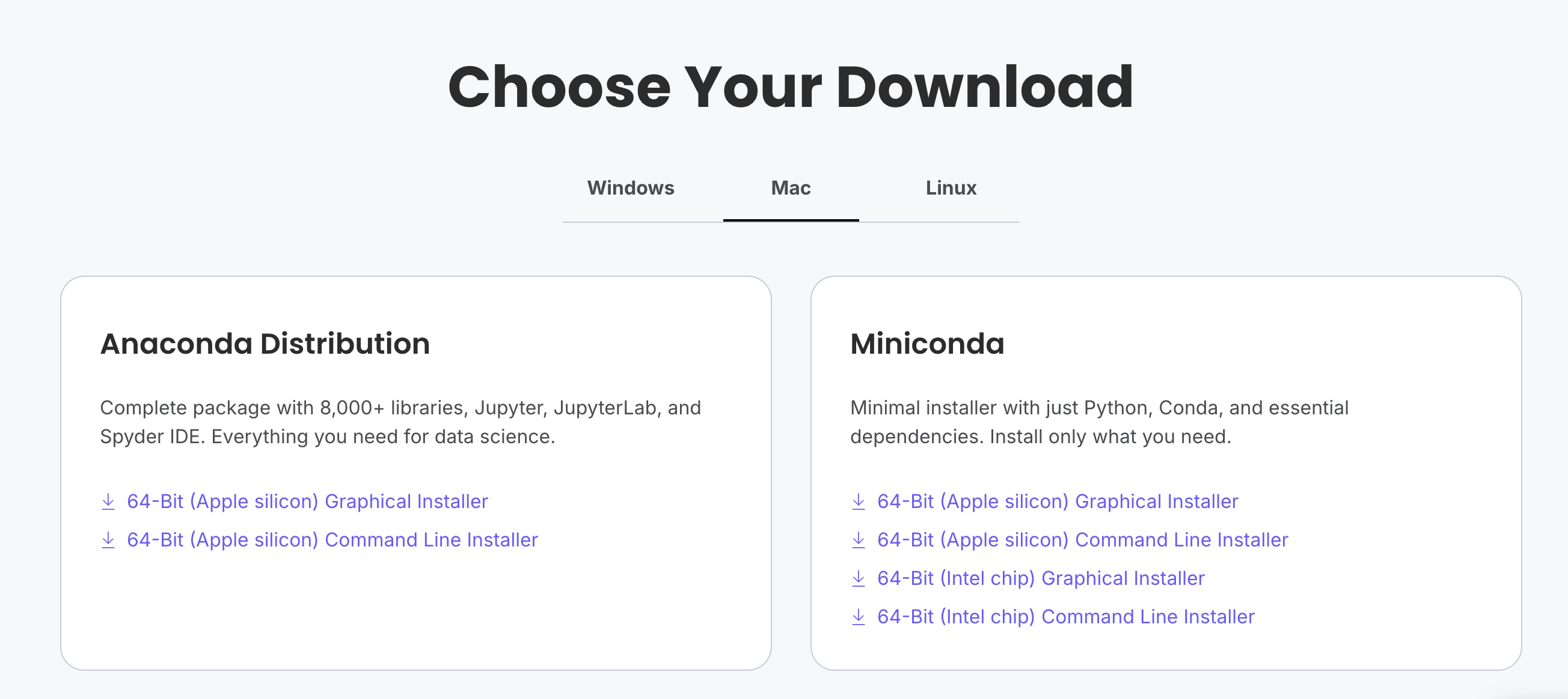
0.3.1 Option 1: Install the Software on Your Computer#
If you choose to install Python locally, we recommend using Miniconda (smaller download) or Anaconda (larger but includes more packages). Both are free and provided by Anaconda Inc.
A conda environment is a self-contained “bubble” that isolates one project (or a group of related projects) from others. Each environment includes its own Python version and a specific set of packages and dependencies, ensuring stable and reproducible workflows.
Key Features
Project Isolation
Each environment is independent. Packages installed in one environment do not affect others or the system-wide Python installation.Dependency Management
Environments prevent conflicts between projects that require different Python or library versions.Version Control
You can create environments with fixed software versions (e.g., Python 3.11) while maintaining others with newer versions.Workflow Management
Start in the default base environment
Activate an environment to work on a project
Deactivate it when finished
Install project-specific libraries (e.g., NumPy, pandas, Jupyter) only within that environment
Analogy
Think of a conda environment as a dedicated toolbox. Each project has its own set of tools, preventing clutter and interference between tasks.
Key takeaway: A conda environment defines what software your code runs with, independently of other projects or the system.
Step 1: Download the Installer#
Choose ONE of these options:
Miniconda (recommended)
Smaller download (~50 MB)
Install only what you need
Anaconda (alternative)
Larger download (~500 MB)
Includes many packages pre-installed
Make sure to download the version for your operating system (Windows, macOS, or Linux) and choose Python 3.
Step 2: Install Miniconda#
Download the Miniconda installer: https://www.anaconda.com/download/success
Follow the installation prompts:
Accept the license agreement
Choose installation location (default is usually fine)
Important: When asked about adding to PATH, choose “Add to PATH” or “Register as default Python”
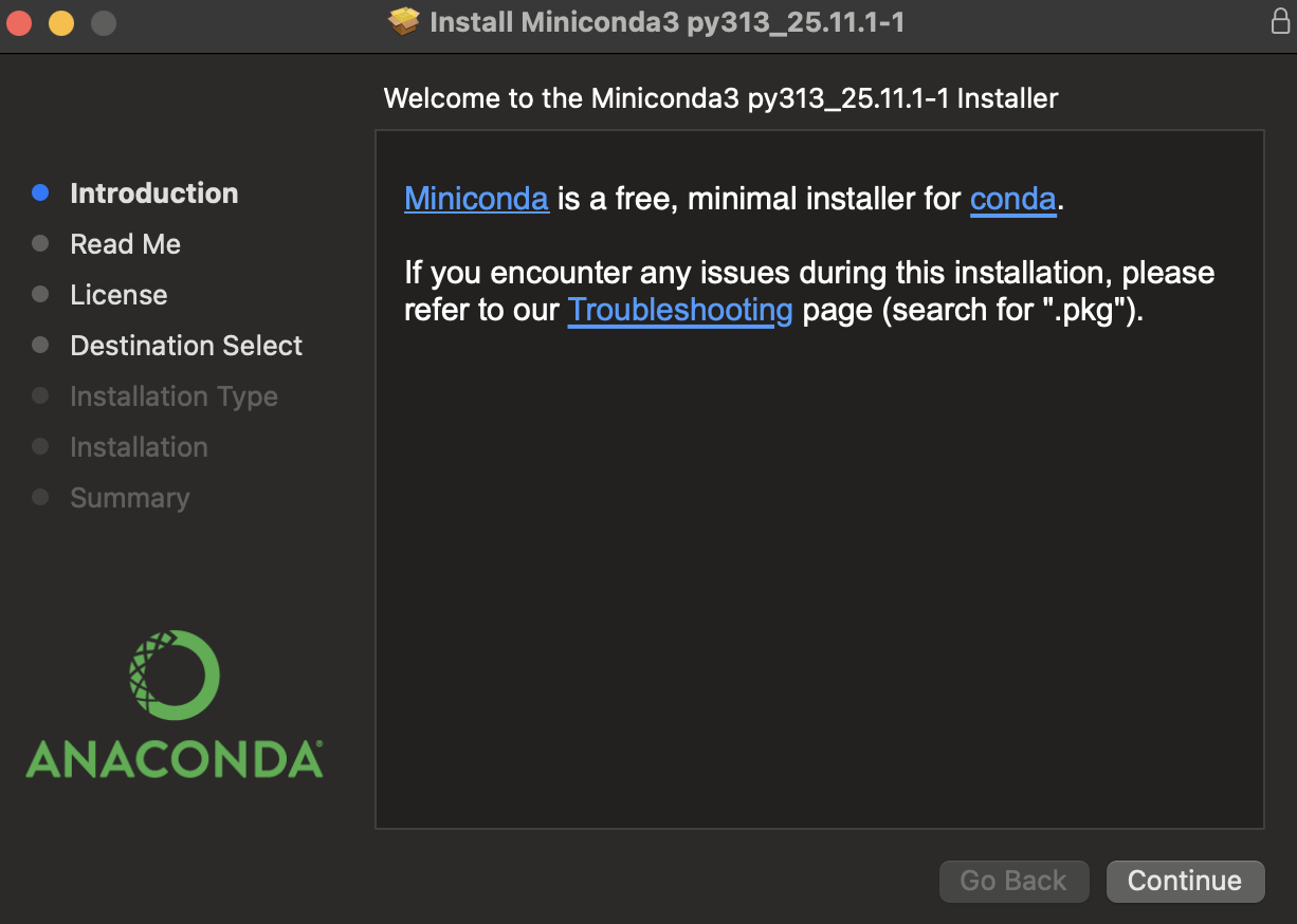
Complete the installation
Step 3: Verify Installation#
Open your Terminal (macOS/Linux) or Command Prompt (Windows) and test that conda is working:
conda --version
You should see a version number like conda 23.x.x.
Step 4: Create a New Environment for This Course#
Create a dedicated environment for this course:
conda create --name chme212 python
This creates a new environment called chme212 with Python installed.
Step 5: Activate Your Environment#
conda activate chme212
You should see (chme212) appear at the beginning of your terminal prompt.
Step 6: Install Required Packages#
You can install all the packages you’ll need for this course using one of these two methods:
Method A: Install packages directly (recommended)
conda install -c conda-forge jupyterlab numpy scipy matplotlib pandas seaborn scikit-learn scikit-image sympy
Note
The conda command installs packages from online repositories called channels. By default, Conda uses the Anaconda channel, which may have licensing restrictions for large organizations (terms here). Adding -c conda-forge tells Conda to use the conda-forge channel instead, which is maintained by the community and free for all users. This is why installation instructions for many packages, such as matplotlib, often include -c conda-forge.
Method B: Install from requirements file
If you have the course requirements.txt file, you can install all packages at once:
pip install -r requirements.txt
Both methods install everything you need. Method A uses conda-forge (which is free for everyone), while Method B uses pip with the course requirements file.
Tip
You can simplify package installation by using a requirements file. This is a plain text file (e.g., requirements.txt) listing all packages, one per line.
Step 7: Register Your Environment with Jupyter#
This allows you to select your chme212 environment when creating notebooks:
python -m ipykernel install --user --name chme212 --display-name "chme212"
Step 8: Launch JupyterLab#
jupyter-lab
JupyterLab will open in your web browser. When creating a new notebook, select chme212 as your kernel. Note that JupyterLab is not a website—the browser is just used as an interface to view and interact with your files locally.
That’s it! You now have a complete Python environment ready for this course.
Important Note: Every time you want to work on course materials, remember to activate your environment first with
conda activate chme212before runningjupyter-lab.
0.3.2 [Optional] Option 2: Use Google Colab#
Google Colab is an easy way to run Python without installing anything on your computer.
All the code runs on Google’s servers, and you access it through your web browser.
To use Colab, you need a free Google account.
If you already use Gmail or your school email is run by Google, you already have one.
Below is the recommended way to set up Colab through Google Drive, so you can save your notebooks and data files easily.
Step 1. Log into Google#
Go to https://google.com
Sign in, or create a free account if needed.
Step 2. Open Google Drive#
Click the Google Apps icon (the 3×3 grid of dots in the top-right corner).
Select Drive.
Step 3. Install the Google Colab Add-on#
This allows you to open Jupyter notebooks directly from Drive.
In Google Drive, look to the right side of the screen.
Click the Get Add-ons button (the + symbol).
In the search bar, type Google Colab or Colaboratory.
Click Install.
Note:
If you already have a.ipynbnotebook in Google Drive, double-clicking it may automatically install the Colab add-on.
Tip:
If Colab doesn’t appear as an option right away, refresh your Google Drive page.
Using Google Colab#
Once the add-on is installed, you can:
Right-click inside Google Drive → New → More → Colaboratory,
orDouble-click any
.ipynbfile to open it in Colab.
Most scientific libraries needed for this course—NumPy, SciPy, Pandas, Seaborn, scikit-image, scikit-learn—are already installed by default.
Installing Extra Libraries (If Needed)#
If a chapter requires a package that is not already included, you can install it by adding this line at the top of your notebook:
!pip install <library>
Using Notebooks in Google Colab#
Google Colab works very similarly to Jupyter Notebook, except everything runs on Google’s servers.
To open an existing notebook (.ipynb):
Simply double-click the file in your Google Drive. It will open automatically in Colab.To create a new notebook:
Click New (top left of Google Drive) → More → Google Colaboratory.
Once your notebook is open, you can run code or Markdown cells using any of the following:
Click the ▶ (Run) button to the left of a cell (Figure 9)
Use the Runtime → Run all option from the top menu
Use the keyboard shortcut Shift + Return
Running a code cell executes the code and displays the output (text, numbers, plots, etc.) directly below the cell.
Running a Markdown cell renders formatted text, math, and headings.
Note: Writing Python code in a Markdown cell will not execute it.
To add new cells:
Click + Code for a new code cell
Click + Text for a new Markdown cell (both buttons appear at the top-left above your notebook)
Accessing Files on Your Google Drive (Important)#
If you want your Colab notebook to load or save files on your Google Drive
(e.g., datasets, images, project files), you must “mount” your Drive inside Colab.
Add the following lines at the top of your notebook:
from google.colab import drive
drive.mount('/content/drive')

%cd /content/drive/My Drive/project
0.4 Using Jupyter Notebooks#
The Jupyter notebook is an interactive document that lets you write and run code, explain your work, and see results—all in one place. A notebook can include live Python code, math equations, explanatory text, images, and plots. Throughout this course, we will use Jupyter notebooks to run examples, perform calculations, and visualize data. Although the notebooks are designed for use in Jupyter, most code will also run in other environments such as an IPython terminal.
A Jupyter notebook is organized into cells, which come in two main types:
Code cells:
These contain Python code. When you run a code cell, the output (numbers, text, figures, etc.) appears right below it.Markdown cells:
These contain explanations, notes, equations, and images. Markdown cells help you describe what your code is doing or present results clearly. They support Markdown formatting, HTML, and LaTeX for mathematical expressions.
print('hello world')
hello world
print(1)
1
0.4.1 Markdown#
Markdown is a simple way to format text in your notebook cells. It lets you make text bold, italic, add headers, create lists, and more—without needing to know complicated formatting codes.
Think of Markdown like shortcuts for formatting. Instead of clicking buttons to make text bold, you just put ** around the words you want to emphasize.
Here are the most useful Markdown commands you’ll need for this course:
Table 1 Essential Markdown Syntax
What You Type |
What You Get |
|---|---|
|
# Big Header |
|
## Medium Header |
|
### Small Header |
|
bold text |
|
italic text |
|
|
|
(horizontal line) |
|
• Item 1 |
|
1. First item |
|
Try It Yourself: Markdown Examples
Important: The cells below show you Markdown formatting in action. Double-click on any of these cells to see the “raw” Markdown code, then press Shift+Enter to see the formatted result.
Example 1: Basic Formatting
If you want to show example Python code in a Markdown cell (without running it), put it between triple backticks with “python”:
~~~python
print("This is example code that won't run")
x = 5 + 3
~~~
This text shows bold formatting, italic formatting, and code formatting.
Here’s a math equation: \(E = mc^2\)
And here’s a link to Google.
Example 2: Headers and Lists
This is a Medium Header#
This is a Small Header#
Bulleted List:
First item
Second item
Third item
Numbered List:
Step one
Step two
Step three
Example 3: Showing Code in Markdown
Sometimes you want to show Python code as an example without running it:
# This code will be displayed with syntax highlighting
import numpy as np
x = np.array([1, 2, 3, 4, 5])
print(f"The average is {np.mean(x)}")
You can also mention short code snippets like print("Hello!") or x = 5 within regular text.
print(‘hello world’)
Your Turn: Practice Cell
Double-click this cell and try editing it! Add your name, make some text bold, create a list of your favorite foods, or write a short explanation of what you learned today.
Remember: Press Shift+Enter when you’re done editing to see the formatted result.
0.5 Overview of Python Scientific Libraries#
The Python programming language allows you to install add-on tools known as libraries or packages that provide additional features. Each library contains one or more modules, and each module contains useful functions (and sometimes datasets).
Here’s how this hierarchy works:
🐍 Python
    └── 📚 Library (e.g., SciPy)
        └── 📄 Module (e.g., integrate)
            └── ⚙️ Function (e.g., quad, trapz)
Example:
Python → SciPy Library → integrate module → quad() function
scipy.integrate.quad()- integrates equations numerically
# Example: Python → SciPy Library → integrate module → quad() function
import scipy.integrate
import numpy as np

# Define a simple function to integrate: f(x) = x^2
def f(x):
    return x**2

# Use scipy.integrate.quad() to integrate from 0 to 2
result, error = scipy.integrate.quad(f, 0, 2)

print(f"Integral of x² from 0 to 2 = {result:.3f}")
print(f"Expected result: 8/3 = {8/3:.3f}")
Integral of x² from 0 to 2 = 2.667
Expected result: 8/3 = 2.667
For scientific and engineering work, Python has a powerful ecosystem of libraries. A core group of these is often referred to as the SciPy stack, but many additional libraries are widely used in chemistry, chemical engineering, and materials science. The table below lists commonly used libraries, with an asterisk indicating those typically considered part of the SciPy stack.
Common Python Libraries for Scientific Computing, including Chemical Engineering, Chemistry, and Materials Science
Library |
Description |
|---|---|
NumPy |
Core library for numerical computing; provides arrays, linear algebra tools, and mathematical functions |
SciPy |
Tools for optimization, integration, interpolation, signal processing, linear algebra, and solving scientific problems |
Matplotlib |
Foundational plotting library for creating graphs and figures |
Scikit-Image |
Tools for scientific image analysis (microscopy, SEM/TEM images, particle analysis, etc.) |
Seaborn |
High-level statistical plotting built on top of Matplotlib |
SymPy |
Symbolic mathematics (similar to Mathematica) |
Pandas |
Data analysis and table (DataFrame) manipulation |
Scikit-Learn |
Machine learning library for classification, regression, clustering, and more |
TensorFlow / PyTorch |
Deep learning frameworks widely used for neural networks |
RDKit |
Cheminformatics toolkit for molecular structures, descriptors, fingerprints, and chemical reactions |
ASE (Atomic Simulation Environment) |
Tools for building atomic structures, running simulations, and analyzing computational chemistry outputs |
pymatgen |
Materials analysis library for DFT calculations, crystal structures, defect chemistry, and phase diagrams |
MDAnalysis |
Analysis of molecular dynamics (MD) trajectories (LAMMPS, GROMACS, AMBER, etc.) |
OpenMM |
Molecular simulation toolkit for running MD simulations directly in Python |
Scikit-Bio |
Computational biology tools (microbiome analysis, sequences, statistics) |
PyTorch Geometric |
Graph neural network toolkits (useful for molecules, materials graphs) |
LAMMPS Python Interface |
Python bindings for controlling LAMMPS molecular dynamics runs |
Adapted from Scientific Computing for Chemists with Python
0.6 Environment Check#
We created a conda environment that includes the required python packages. Let’s make sure everything is working! Run the cell below:
What is a Python Environment? A Python environment is like a separate workspace that contains a specific version of Python and a specific set of packages. Think of it like having different toolboxes for different projects:
Your
chme212environment has all the scientific computing tools we need (NumPy, Matplotlib, etc.)Your base environment might have different packages
This keeps projects organized and prevents conflicts between package versions
What is a Jupyter Kernel?
A Jupyter kernel is the “engine” that runs your Python code in the notebook. When you select a kernel (like chme212), you’re telling Jupyter:
Which Python environment to use
Which packages are available
Where to run your code
Why This Matters: If you select the wrong kernel, you might get “module not found” errors because the packages aren’t installed in that environment. Always make sure you’re using the chme212 kernel for this course!
# Environment Check - Run this first!
import sys
print(f"✅ Python version: {sys.version}")
print(f"✅ You're running Python from: {sys.executable}")
print("\n🎉 Great! Your Python environment is working!")
✅ Python version: 3.10.18 | packaged by conda-forge | (main, Jun  4 2025, 14:46:00) [Clang 18.1.8 ]
✅ You're running Python from: /Users/hoon/miniconda3/envs/chemcomp/bin/python

🎉 Great! Your Python environment is working!
# Check installed packages and their versions
import importlib.metadata

# List of packages we commonly use in this course
packages = ['numpy', 'matplotlib', 'pandas', 'scipy', 'seaborn', 'scikit-learn', 'sympy']

print("Package Version Check:")
print("=" * 40)

for package in packages:
    try:
        version = importlib.metadata.version(package)
        print(f"{package:<15} {version} Installed!")
    except importlib.metadata.PackageNotFoundError:
        print(f"{package:<15} NOT INSTALLED!")

print("\n Alternative method - using __version__ attribute:")
print("=" * 50)

# Alternative method for some packages
import numpy as np
import matplotlib
try:
    import pandas as pd
    print(f"NumPy:      {np.__version__}")
    print(f"Matplotlib: {matplotlib.__version__}")
    print(f"Pandas:     {pd.__version__}")
except ImportError as e:
    print(f"Import error: {e}")

print(f"\n If any packages are missing, you can install them using:")
print(f"   conda install -c conda-forge <package-name>")
print(f"   or: pip install <package-name>")
Package Version Check:
========================================
numpy           1.26.4 Installed!
matplotlib      3.10.8 Installed!
pandas          2.3.3 Installed!
scipy           1.15.2 Installed!
seaborn         0.13.2 Installed!
scikit-learn    1.7.2 Installed!
sympy           1.14.0 Installed!

 Alternative method - using __version__ attribute:
==================================================
NumPy:      1.26.4
Matplotlib: 3.10.8
Pandas:     2.3.3

 If any packages are missing, you can install them using:
   conda install -c conda-forge <package-name>
   or: pip install <package-name>
0.4.2 Comments#
Comments help you remember what your code does. What seems obvious today won’t be obvious in a week!
Use the
#symbol to add comments to your code. Everything after#on a line is ignored when the code runs.You can comment an entire line or add a comment at the end of a line of code: